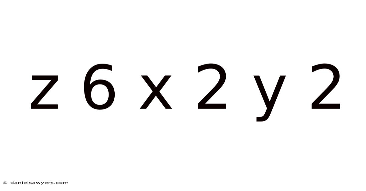
Understanding the Multivariable Function $z = 6x^2y^2$: Analysis, Graphing, and Calculus Applications
The mathematical expression $z = 6x^2y^2$ represents a scalar-valued function of two variables, a fundamental concept in multivariable calculus and three-dimensional analytic geometry. Here's the thing — while the notation "z 6 x 2 y 2" appears as a linear string of characters, standard mathematical convention interprets this as $z = 6x^2y^2$, where the coefficient 6 multiplies the squared terms of both independent variables $x$ and $y$. This function defines a surface in three-dimensional space ($\mathbb{R}^3$) that exhibits unique symmetry properties, critical point behavior, and applications in optimization problems. This article provides a comprehensive exploration of this function, covering its algebraic structure, geometric visualization, differential calculus properties, and practical significance Surprisingly effective..
Algebraic Structure and Domain Analysis
At its core, $f(x, y) = 6x^2y^2$ is a polynomial function of degree four (quartic). Unlike linear or quadratic forms (degree 1 or 2), this function grows at a rate proportional to the fourth power of the distance from the origin.
Domain and Range The domain of this function is the entire Cartesian plane, $\mathbb{R}^2$. There are no restrictions such as division by zero, square roots of negative numbers, or logarithmic constraints. Any real number pair $(x, y)$ produces a valid real output $z$.
The range, however, is restricted. Since $x^2 \ge 0$ and $y^2 \ge 0$ for all real $x, y$, their product $x^2y^2$ is also non-negative. Multiplying by the positive constant 6 preserves this inequality. So, the range is $z \in [0, \infty)$. Consider this: the absolute minimum value of the function is $z = 0$, achieved along the entire $x$-axis ($y=0$) and the entire $y$-axis ($x=0$). There is no absolute maximum; the function increases without bound as $|x|$ or $|y|$ increase Simple, but easy to overlook..
Counterintuitive, but true.
Symmetry Properties The function possesses significant symmetry, which simplifies both analysis and graphing:
- Even Symmetry in $x$: $f(-x, y) = 6(-x)^2y^2 = 6x^2y^2 = f(x, y)$. The surface is symmetric with respect to the $yz$-plane.
- Even Symmetry in $y$: $f(x, -y) = 6x^2(-y)^2 = 6x^2y^2 = f(x, y)$. The surface is symmetric with respect to the $xz$-plane.
- Rotational Symmetry (Quadrant Symmetry): Because the function depends only on the squares of the variables, the surface in all four quadrants of the $xy$-plane is identical. Analyzing the first quadrant ($x \ge 0, y \ge 0$) fully describes the entire surface.
Geometric Visualization: The Shape of the Surface
Visualizing $z = 6x^2y^2$ requires understanding its cross-sections (traces) and level curves (contour lines) Not complicated — just consistent..
Traces (Cross-Sections)
- Trace in $x=0$ (the $yz$-plane): $z = 6(0)^2y^2 = 0$. This is the $y$-axis.
- Trace in $y=0$ (the $xz$-plane): $z = 6x^2(0)^2 = 0$. This is the $x$-axis.
- Trace in $y = k$ (constant): $z = 6k^2x^2$. For any non-zero constant $k$, this is a parabola opening upward in the $xz$-plane with vertex at the origin. The "width" of the parabola is controlled by $6k^2$; larger $|k|$ creates a steeper, narrower parabola.
- Trace in $x = k$ (constant): $z = 6k^2y^2$. Similarly, this yields upward-opening parabolas in the $yz$-plane.
- Trace in $z = c$ (horizontal planes, $c > 0$): $c = 6x^2y^2 \implies x^2y^2 = \frac{c}{6} \implies |xy| = \sqrt{\frac{c}{6}}$. This describes four hyperbolas in the plane $z=c$, asymptotic to the coordinate axes.
Level Curves (Contour Map) Level curves are the projections of the horizontal traces onto the $xy$-plane. Setting $z = k$ (where $k \ge 0$): $6x^2y^2 = k \implies x^2y^2 = \frac{k}{6} \implies xy = \pm \sqrt{\frac{k}{6}}$ For $k=0$, the level "curve" degenerates into the union of the $x$ and $y$ axes (the coordinate cross). For $k > 0$, the level curves are rectangular hyperbolas centered at the origin with
their asymptotes along the coordinate axes. As $k$ increases, these hyperbolas move further away from the origin, reflecting the function's unbounded growth Easy to understand, harder to ignore..
Behavior Near Critical Features
The function exhibits distinct behavior near its critical features. Plus, along the coordinate axes, where either $x=0$ or $y=0$, the function remains identically zero, creating a valley that extends infinitely along both axes. Moving away from the axes into any quadrant, the function increases rapidly due to the quartic nature of the expression. The rate of increase accelerates as both $|x|$ and $|y|$ grow, since the product $x^2y^2$ involves fourth-order terms And that's really what it comes down to..
Comparison with Related Functions
Comparing $z = 6x^2y^2$ to simpler functions like $z = x^2 + y^2$ (a circular paraboloid) or $z = x^2 - y^2$ (a hyperbolic paraboloid) reveals important distinctions. While the sum $x^2 + y^2$ creates radial symmetry with circular level curves, the product $x^2y^2$ generates the more complex rectangular hyperbolic level curves. Unlike the saddle point of $z = x^2 - y^2$, the origin here represents a global minimum, but the valley structure is one-dimensional rather than point-like Most people skip this — try not to..
Applications and Modeling
Functions of the form $z = ax^2y^2$ appear naturally in various physical and optimization contexts. Worth adding: they model phenomena where the effect depends multiplicatively on two squared variables, such as certain stress-strain relationships in materials science or interaction energies in statistical mechanics. The symmetry properties make them particularly useful in problems where the influence of two perpendicular directions combines multiplicatively.
Conclusion
The function $z = 6x^2y^2$ demonstrates how simple algebraic operations can generate complex geometric structures. That's why its non-negative range $[0, \infty)$, extensive symmetry properties, and distinctive level curves of rectangular hyperbolas make it a compelling example in multivariable calculus. The absence of an absolute maximum alongside the presence of an absolute minimum along entire lines illustrates that extrema need not be isolated points. Understanding such functions provides essential intuition for analyzing more complex surfaces encountered in advanced mathematics, physics, and engineering applications.
Gradient, Critical Manifold, and Second‑Order Test
The partial derivatives of (z = 6x^{2}y^{2}) are
[ \frac{\partial z}{\partial x}=12xy^{2},\qquad \frac{\partial z}{\partial y}=12x^{2}y . ]
Setting both components to zero yields the condition (xy=0); consequently every point on the coordinate axes is a critical point. Unlike functions that possess isolated stationary points, this one has a one‑dimensional critical manifold that stretches infinitely in both directions That's the part that actually makes a difference..
The Hessian matrix,
[ H=\begin{pmatrix} 12y^{2} & 12xy\[2pt] 12xy & 12x^{2} \end{pmatrix}, ]
has determinant
[ \det H = 144x^{2}y^{2}-144x^{2}y^{2}=0, ]
so the usual second‑derivative test is inconclusive off the axes. Worth adding: along the axes the function is identically zero, while any departure from those lines produces a strictly positive value. Despite this, the sign of the quadratic form (6x^{2}y^{2}) makes it clear that the surface never takes negative values. Hence the entire (x)- and (y)-axes constitute a global minimum set, and the surface can be viewed as a “valley” that is flat precisely on those lines.
Homogeneity and Scaling
The expression is homogeneous of degree four: scaling the variables by factors (a) and (b),
[ z(ax,by)=6(ax)^{2}(by)^{2}=a^{2}b^{2},6x^{2}y^{2}=a^{2}b^{2},z(x,y). ]
This property explains why the level curves expand rapidly as the parameter (k) grows; doubling both coordinates multiplies the height by a factor of four, while doubling only one coordinate multiplies the height by two.
Qualitative Shape and Topological Features
Because the function depends on the product of two squares, the surface is symmetric with respect to the planes (x=0), (y=0), (x=y), and (x=-y). The graph therefore consists of four identical “wings” that rise from the flat valley on the axes and bend outward in the diagonal directions. If one projects the surface onto the (xy)-plane, the silhouette is a cross formed by the axes; the three‑dimensional shape resembles a pair of opposing “saddles” that are glued together along the entire coordinate lines Most people skip this — try not to..
A useful mental model is obtained by introducing the variables
[ u = x^{2},\qquad v = y^{2}, ]
which map the first quadrant onto the first quadrant of the (uv)-plane. In these new coordinates the function becomes
[ z = 6uv, ]
the equation of a hyperbolic paraboloid in the ((u,v))-space. Pulling this surface back through the square‑root transformation yields the rectangular hyperbolas that appear as level sets in the original ((x,y))-plane That alone is useful..
Visualization and Computational Insight
A quick script that samples the function on a grid and draws the corresponding contours reveals the rectangular hyperbolas more clearly than a wire‑frame view of the surface itself. By coloring each contour according to its value, one observes that the spacing between successive curves widens as the distance from the origin increases, reflecting the accelerating growth of the function. This visual cue reinforces the analytical observation that the rate of increase is governed by the fourth‑order term (x^{2}y^{2}).
Concluding Remarks
The simple polynomial (z = 6x^{2}y^{2}) showcases how modest algebraic ingredients can generate a rich geometric picture: a non‑negative surface bounded below by a one‑dimensional minimum set, an absence of any finite upper bound, and a family of level curves that are rectangular hyperbolas. That said, its symmetry, homogeneity, and the nature of its critical manifold make it an instructive exemplar in multivariable calculus, illustrating concepts such as constrained extrema, homogeneity, and the behavior of level sets. Understanding these properties provides a solid foundation for tackling more layered surfaces that arise in physics, engineering, and optimization problems Turns out it matters..
