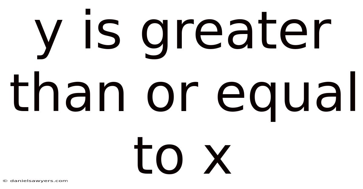
Understanding the relationship between variables is the cornerstone of algebra, calculus, and mathematical modeling. This expression asserts that the value of the dependent variable y is either strictly larger than the independent variable x or exactly identical to it. That's why the statement y is greater than or equal to x, written symbolically as y ≥ x, represents a fundamental inequality that defines a specific region in the coordinate plane and governs constraints in optimization problems. Mastering this concept unlocks the ability to graph solution sets, solve systems of constraints, and interpret real-world scenarios where minimum thresholds are required Surprisingly effective..
The Symbolism and Basic Definition
The symbol ≥ combines the "greater than" symbol (>) with a line underneath representing "equal to" (=). When we write y ≥ x, we are making a compound statement: y > x OR y = x. Both conditions satisfy the inequality Easy to understand, harder to ignore. Nothing fancy..
Unlike an equation such as y = x, which describes a single, infinitely thin line, an inequality describes a half-plane—a vast region containing infinite coordinate pairs. For every possible x value, there is a corresponding range of y values that make the statement true. If x = 3, then y can be 3, 4, 5, 100, or 3.0001. The only values that fail are those strictly less than 3 Took long enough..
Graphical Representation: Visualizing the Half-Plane
Graphing y ≥ x provides an immediate visual intuition that algebraic manipulation alone cannot offer. The process involves three distinct steps:
- Graph the Boundary Line: First, treat the inequality as an equation: y = x. This is a straight line passing through the origin (0,0) with a slope of 1. Because the inequality includes "equal to" (≥), the boundary line is drawn as a solid line. A dashed or dotted line would be used for strict inequalities (y > x), indicating the line itself is not part of the solution.
- Select a Test Point: Choose a coordinate pair not on the line to determine which side of the boundary to shade. The origin (0,0) lies on the line y = x, so it cannot be used. A convenient alternative is (0, 1) or (1, 0).
- Test and Shade: Substitute the test point into the original inequality.
- Testing (0, 1): Is 1 ≥ 0? Yes. This point satisfies the condition.
- Testing (1, 0): Is 0 ≥ 1? No. This point fails. Since (0, 1) works, we shade the region above the line (the side containing the positive y-axis). This shaded area, including the solid line itself, represents every solution to y ≥ x.
Key Visual Takeaway: The solution set is the "upper" half-plane relative to the diagonal line y = x.
Algebraic Manipulation and Properties
Working with y ≥ x algebraically requires adherence to the Properties of Inequalities. These rules dictate how the relationship changes when operations are applied to both sides Easy to understand, harder to ignore..
- Addition/Subtraction Property: You can add or subtract any real number c to both sides without changing the direction of the inequality.
- y + 5 ≥ x + 5 is equivalent to y ≥ x.
- Multiplication/Division Property (Positive Numbers): Multiplying or dividing by a positive number preserves the inequality direction.
- 2y ≥ 2x simplifies to y ≥ x.
- Multiplication/Division Property (Negative Numbers) — Critical Rule: Multiplying or dividing by a negative number reverses the inequality symbol.
- -y ≥ -x becomes y ≤ x (after multiplying by -1).
- This is the most common source of errors in algebraic problem solving.
Rearranging Forms: The inequality y ≥ x is often rewritten to fit standard forms used in linear programming or calculus:
- Standard Form: y - x ≥ 0 or -x + y ≥ 0.
- Slope-Intercept Form: y ≥ 1x + 0 (slope m=1, y-intercept b=0).
Systems of Inequalities: The Feasible Region
In advanced applications—particularly linear programming—y ≥ x rarely exists in isolation. It functions as a constraint within a system of inequalities. The solution to the system is the intersection of the half-planes defined by each inequality, known as the feasible region Surprisingly effective..
And yeah — that's actually more nuanced than it sounds.
Consider a system modeling a production scenario:
- y ≥ x (Product B output must be at least Product A output)
- x + y ≤ 100 (Total capacity limit)
Graphing these together creates a polygonal feasible region. The vertices (corner points) of this polygon are candidates for optimal solutions (maximum profit or minimum cost) according to the Corner Point Theorem. The line y = x acts as a diagonal boundary cutting through the first quadrant, restricting solutions to those where y dominates x.
It sounds simple, but the gap is usually here.
Real-World Applications and Contextual Meaning
The abstraction y ≥ x translates directly into tangible "minimum requirement" scenarios across diverse fields Which is the point..
Economics and Budgeting
Imagine a household budget where x represents spending on "wants" (entertainment, dining out) and y represents spending on "needs" (rent, utilities, savings). A financial advisor might impose the rule y ≥ x. This ensures the household never spends more on discretionary items than on essential obligations. If x = $500, then y must be at least $500 Still holds up..
Engineering and Safety Factors
In structural engineering, x might represent the applied load (stress) on a beam, and y represents the yield strength (capacity) of the material. The safety constraint is y ≥ x (often with a safety factor multiplier, e.g., y ≥ 1.5x). If the load exceeds the strength (x > y), structural failure occurs. The inequality defines the safe operating envelope.
Computer Science and Algorithms
In algorithm analysis, y ≥ x appears in loop invariants and correctness proofs. To give you an idea, in a binary search, the index of the high pointer (y) must always be greater than or equal to the low pointer (x) for the search space to be valid. If y < x, the search space is empty, and the algorithm terminates Simple, but easy to overlook..
Data Science and Machine Learning
In ranking algorithms or recommendation systems, a constraint y ≥ x might enforce that a "premium" content score (y) is never lower than a "standard" content score (x) for the same user query, ensuring business logic consistency That's the part that actually makes a difference..
The "Equal To" Component: Boundary Solutions
The inclusion of "equal to" (≥ vs >) is mathematically significant. It changes the topology of the solution set.
- Closed Set: y ≥ x defines a closed set in topology. It contains all its boundary points (the line y = x). This guarantees the existence of minimum or maximum values for continuous functions over this domain (via the Extreme Value Theorem), provided the domain is also bounded.
- Open Set: y > x defines an open set. The boundary line is excluded. A continuous function on an open,
When the inequality is strict, the feasible region lacks the “edge” where a optimum might sit, and the theorem no longer guarantees a solution. In such cases, the analysis must shift to examining limiting behavior: as the variables approach the excluded boundary, the objective function may approach a supremum or infimum, but without the boundary itself the extreme values remain unattainable. This subtlety is why many real‑world formulations deliberately embed the “equal to” clause, ensuring that the set is closed and that standard optimization techniques—such as linear programming simplex or the Karush‑Kuhn‑Tucker conditions—can be applied with confidence.
The corner‑point theorem therefore serves as a bridge between abstract geometry and concrete decision‑making. Which means by restricting attention to the vertices of the polygon, analysts can reduce an potentially infinite search space to a finite set of candidates, dramatically simplifying computation. This leads to in economics, for example, the intersection of the budget line with the requirement line often yields the most efficient allocation; in engineering, the point where load equals yield strength marks the threshold of failure, a critical benchmark for safety assessments; in computer science, the moment when the high and low indices converge signals the termination condition of a search algorithm. Each of these applications benefits from the certainty that the optimum, if it exists, will be found among the corner points of the feasible polygon.
Some disagree here. Fair enough.
Beyond the mathematical elegance, the presence of the equality component carries practical implications. It forces designers to consider the boundary case explicitly, prompting a sanity check that the system can tolerate the minimal acceptable level of performance. In budgeting, this translates to a policy that never permits discretionary spending to outpace essential expenditures, thereby safeguarding financial stability. In structural design, specifying that the safety margin must be at least equal to the applied load ensures that engineers allocate sufficient material to absorb unexpected surges, reducing the risk of catastrophic overload. In algorithmic contexts, enforcing that the high pointer be greater than or equal to the low pointer prevents infinite loops and guarantees termination.
To keep it short, the inequality y ≥ x is more than a simple arithmetic expression; it encapsulates a fundamental principle of feasibility—any viable solution must meet a minimum threshold. In practice, the Corner Point Theorem leverages the geometric properties of the resulting polygon to pinpoint where optimal outcomes reside, while the inclusion of “equal to” guarantees that the search space is closed, allowing both existence proofs and efficient computational methods to be employed. By recognizing the interplay between mathematical rigor and real‑world constraints, practitioners across economics, engineering, computer science, and data science can harness this framework to devise solid, reliable, and efficient solutions.
