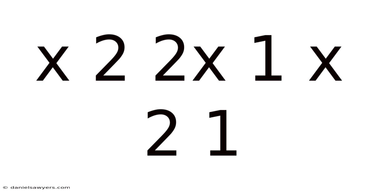
Understanding the Quadratic Expression (x^{2}+2x+1)
At first glance the string “x 2 2x 1 x 2 1” might look like a jumble of symbols, but when we interpret the spaces as missing operators it becomes the familiar quadratic expression
[ x^{2}+2x+1 . ]
This simple polynomial appears repeatedly in algebra, calculus, and even real‑world modeling. Practically speaking, in the sections that follow we will break down every aspect of (x^{2}+2x+1): its structure, factoring, roots, graph, practical uses, and common pitfalls. Consider this: though it may seem elementary, mastering its properties builds a solid foundation for tackling more complex equations. By the end you should feel comfortable recognizing, manipulating, and applying this expression in a variety of contexts.
1. Breaking Down the Components
A quadratic expression generally takes the form
[ ax^{2}+bx+c, ]
where (a), (b), and (c) are constants and (x) is the variable. For (x^{2}+2x+1) we can identify:
| Symbol | Value | Role |
|---|---|---|
| (a) | 1 | Coefficient of the (x^{2}) term |
| (b) | 2 | Coefficient of the linear (x) term |
| (c) | 1 | Constant term |
Because (a=1), the quadratic is monic—its leading coefficient equals one. This property often simplifies factoring and completing the square That's the whole idea..
2. Factoring the Expression
2.1 Recognizing a Perfect Square Trinomial
A perfect square trinomial follows the pattern
[ (p+q)^{2}=p^{2}+2pq+q^{2}. ]
If we set (p=x) and (q=1), we obtain
[ (x+1)^{2}=x^{2}+2\cdot x\cdot1+1^{2}=x^{2}+2x+1. ]
Thus, (x^{2}+2x+1) is a perfect square and factors neatly as
[ \boxed{(x+1)^{2}}. ]
2.2 Alternative Factoring Methods
Even if the perfect‑square pattern isn’t immediately obvious, you can factor by:
- Trial and error – look for two numbers that multiply to (a\cdot c = 1) and add to (b = 2). The pair (1, 1) works, giving the factors ((x+1)(x+1)).
- Quadratic formula – solving (ax^{2}+bx+c=0) yields roots (x = \frac{-b\pm\sqrt{b^{2}-4ac}}{2a}). Plugging in (a=1, b=2, c=1) gives a double root at (x=-1), confirming the factor ((x+1)) appears twice.
3. Solving the Equation (x^{2}+2x+1=0)
Setting the expression equal to zero leads to:
[ x^{2}+2x+1=0 ;\Longrightarrow; (x+1)^{2}=0. ]
Taking the square root of both sides yields:
[ x+1=0 \quad\Rightarrow\quad x=-1. ]
Because the factor is squared, (-1) is a double root (also called a repeated root). Graphically, the parabola touches the x‑axis at this point but does not cross it.
4. Graphical Interpretation
4.1 Shape and Vertex
The graph of (y = x^{2}+2x+1) is a parabola that opens upward (since (a>0)). Completing the square reveals its vertex form:
[ \begin{aligned} y &= x^{2}+2x+1 \ &= (x^{2}+2x)+1 \ &= (x+1)^{2}. \end{aligned} ]
Thus the vertex is at ((-1,,0)). The axis of symmetry is the vertical line (x=-1).
4.2 Intercepts
- y‑intercept: set (x=0) → (y = 0^{2}+2\cdot0+1 = 1). Point ((0,1)).
- x‑intercept: as shown above, the only x‑intercept is ((-1,0)) (a tangent point).
4.3 Sketch
   y
   ↑
 2 |          *
   |         *
 1 |*        *
   |  *      *
 0 +---*----*----→ x
   -2 -1   0   1
The star at ((-1,0)) marks the vertex and the sole x‑intercept Practical, not theoretical..
5. Applications in Mathematics and Beyond
5.1 Algebraic Manipulations
Because ((x+1)^{2}) expands to (x^{2}+2x+1), the expression is handy for:
- Completing the square in more complex quadratics.
- Simplifying rational expressions where the numerator or denominator contains this trinomial.
- Deriving formulas such as the quadratic formula itself (the discriminant (b^{2}-4ac) becomes zero for this case).
5.2 Calculus
- Derivative: (\frac{d}{dx}(x^{2}+2x+1)=2x+2 = 2(x+1)). The derivative zeroes at (x=-1), confirming the vertex.
- Integral: (\int (x^{2}+2x+1),dx = \frac{x^{3}}{3}+x^{2}+x + C). The antiderivative can be expressed as (\frac{(x+1)^{3}}{3}+C) after substitution.
5.3 Physics and Engineering
Quadratic expressions model phenomena with constant acceleration. Take this: the displacement (s) of an object under uniform acceleration (a) after time (t) with initial velocity (v_{0}) and initial position (s_{0}) is:
[ s = s_{0}+v_{0}t+\frac{1}{2}at^{2}. ]
If we set (s_{0}=0), (v_{0}=2), and (a=2), the displacement simplifies to (s = t^{2}+2t+1 = (t+1)^{2}). Thus the same algebraic structure appears in
