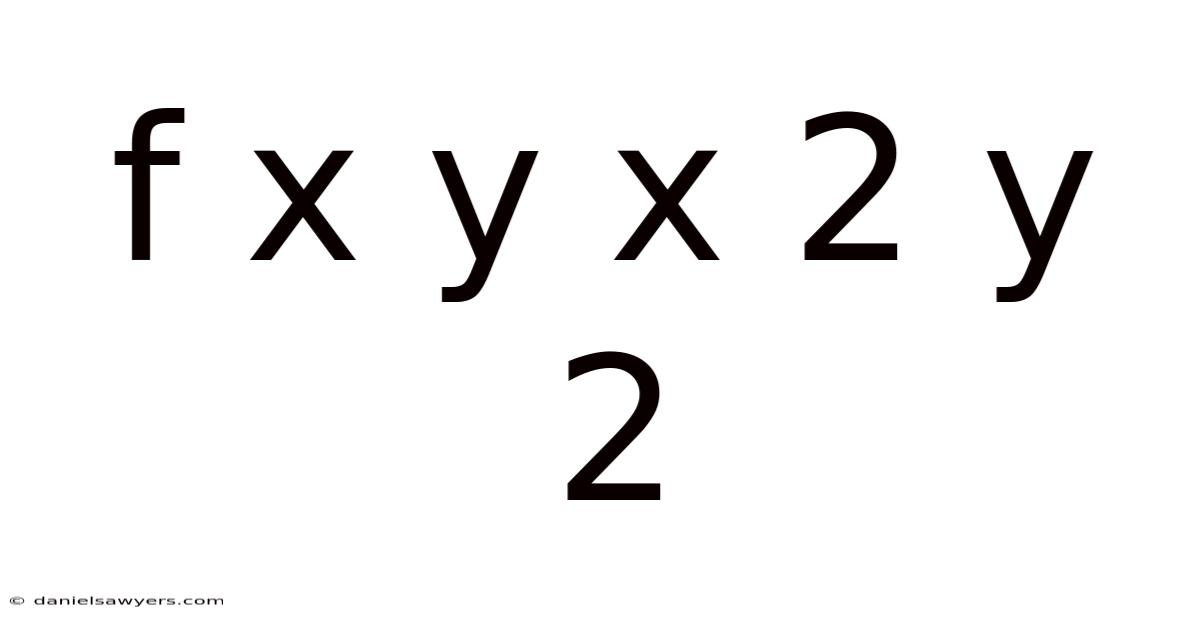
The function f(x, y) = x² + y² is one of the most frequently encountered expressions in multivariable calculus, geometry, and applied mathematics. It represents the sum of the squares of two variables and serves as a simple yet powerful model for distance from the origin, energy in physical systems, and the shape of a circular paraboloid. Consider this: understanding its properties not only builds a solid foundation for more complex functions but also reveals how a basic algebraic form can describe real‑world phenomena ranging from gravitational potential wells to optimization landscapes. This article explores the definition, graphical behavior, mathematical properties, and practical applications of f(x, y) = x² + y², offering step‑by‑step guidance on how to analyze and visualize the surface.
Definition and Basic Characteristics
At its core, f(x, y) = x² + y² is a quadratic form in two variables. Which means as x or y move away from zero, the output grows proportionally to the square of the distance from the origin. For any ordered pair (x, y) in ℝ², the function returns a non‑negative real number because squaring eliminates sign information, and the sum of two non‑negative terms is itself non‑negative. The minimum value occurs at the origin (0, 0), where f(0, 0) = 0. This relationship is why the function is often described as the squared Euclidean distance from (0, 0) to (x, y) And it works..
This changes depending on context. Keep that in mind.
Mathematically, the function can be written as
[ f:\mathbb{R}^2 \rightarrow \mathbb{R}, \qquad f(x,y)=x^{2}+y^{2}. ]
Because both partial derivatives exist and are continuous everywhere, f is differentiable on the entire plane, making it an ideal candidate for applying calculus tools such as gradients and Hessian matrices.
Graphical Representation
2‑D Cross‑Sections
If we fix one variable and plot the resulting single‑variable function, we obtain simple parabolas:
- Setting y = 0 gives f(x, 0) = x², a standard upward‑opening parabola in the x‑z plane.
- Setting x = 0 yields f(0, y) = y², an identical parabola in the y‑z plane.
These cross‑sections illustrate how the function grows symmetrically along each axis.
3‑D Surface
In three dimensions, the set of points (x, y, z) satisfying z = x² + y² forms a circular paraboloid. The surface opens upward, with its vertex at the origin. Because of that, cross‑sections parallel to the xy‑plane are circles: for a constant z = c > 0, the equation x² + y² = c describes a circle of radius √c. As z increases, the radius grows, creating the characteristic “bowl” shape.
Visualizing this surface helps in understanding concepts such as level curves, gradients, and optimization. Level curves (contour lines) are given by x² + y² = k, which are circles centered at the origin with radius √k. These concentric circles are the basis for contour plots used in topography, thermodynamics, and many engineering fields Which is the point..
Mathematical Properties
Gradient and Critical Points
The gradient of f is
[ \nabla f = \left( \frac{\partial f}{\partial x}, \frac{\partial f}{\partial y} \right) = (2x, 2y). ]
Setting the gradient to zero yields the single critical point (0, 0). Because the Hessian matrix
[ H = \begin{pmatrix} 2 & 0 \ 0 & 2 \end{pmatrix} ]
is positive definite (its eigenvalues are both 2 > 0), the critical point is a strict local minimum, which is also the global minimum for this function.
Directional Derivatives
The directional derivative in the direction of a unit vector u = (u₁, u₂) at a point (x, y) is
[ D_{\mathbf{u}}f(x,y) = \nabla f \cdot \mathbf{u} = 2x u_{1} + 2y u_{2}. ]
This shows that the steepest ascent direction is radially outward from the origin, while the steepest descent points directly toward the origin Easy to understand, harder to ignore..
Convexity
Because the Hessian is constant and positive definite, f is convex. Convexity guarantees that any local minimum is also a global minimum, a property that underpins many optimization algorithms, especially in machine learning where f(x, y) serves as a simple loss surface Not complicated — just consistent..
This changes depending on context. Keep that in mind.
Applications in Science and Engineering
-
Physics – Potential Energy
In classical mechanics, the potential energy of a mass attached to a spring in two dimensions can be modeled by a quadratic form similar to x² + y² when the restoring force is isotropic. The function describes a harmonic oscillator potential well. -
Signal Processing – Energy of a Vector
The expression x² + y² is the squared Euclidean norm of a vector (x, y). In signal processing, this norm represents the total energy of a two‑dimensional signal, and minimizing it corresponds to finding the least‑energy solution That's the whole idea.. -
Optimization – Benchmark Function
Researchers often use f(x, y) = x² + y² as a benchmark for testing gradient‑based optimization methods. Its simplicity allows for easy verification of convergence and accuracy. -
Computer Graphics – Distance Fields
Distance fields in graphics frequently rely on squared distance calculations for speed. The function provides a fast way to compute how far a point is from a central point, useful in shading and collision detection That's the whole idea..
Step‑by‑Step Analysis of f(x, y) = x² + y²
1. Identify the Function and Domain
- Function: f(x, y) = x² + y²
- Domain: All real numbers (ℝ²)
2. Compute Partial Derivatives
[ \frac{\partial f}{\partial x}=2x, \quad \frac{\partial f}{\partial y}=2y. ]
3. Find Critical Points
Set both partial derivatives to zero:
2x = 0 → x = 0
2y =
Step 3. Solve the system of equations
[
2x = 0 ;;\Longrightarrow;; x = 0, \qquad
2y = 0 ;;\Longrightarrow;; y = 0 .
]
Thus the only stationary point of (f) in (\mathbb{R}^2) is the origin ((0,0)).
Step 4. Second‑order test
The second partial derivatives are constant: [ \frac{\partial^2 f}{\partial x^2}=2,\qquad \frac{\partial^2 f}{\partial y^2}=2,\qquad \frac{\partial^2 f}{\partial x\partial y}=0 . ]
About the He —ssian matrix is therefore [ H = \begin{pmatrix} 2 & 0\[2pt] 0 & 2 \end{pmatrix}. ]
Because both diagonal entries are positive and (\det(H)=4>0), the Hessian is positive definite. Because of this, the stationary point ((0,0)) is a strict local minimum. In fact, for a quadratic form with a positive‑definite Hessian, this local minimum is automatically the global minimum over the entire domain (\mathbb{R}^2).
Step 5. Gradient‑descent perspective
A simple gradient‑descent iteration for minimizing (f) takes the form
[
\mathbf{z}_{k+1}= \mathbf{z}_k - \alpha \nabla f(\mathbf{z}_k)
= \mathbf{z}_k - \alpha (2x_k, 2y_k),
]
where (\mathbf{z}_k = (x_k, y_k)^\top) and (\alpha>0) is a step size.
On the flip side, choosing (\alpha) smaller than (1/2) guarantees convergence:
[
\mathbf{z}_k ;\xrightarrow{k\to\infty}; (0,0). ]
The convergence is linear and the error decays as (| \mathbf{z}_k| = (1-2\alpha)^k | \mathbf{z}_0|).
Step 6. Connections to broader concepts
-
Quadratic forms – In (n) dimensions, (f(\mathbf{x}) = \mathbf{x}^\top I \mathbf{x}) is the prototypical positive‑definite quadratic form. Its analysis extends directly to ridge‑regression penalties, where the same Hessian governs the curvature of the loss surface The details matter here. Surprisingly effective..
-
Regularization – Adding a term (\lambda|\mathbf{x}|2^2) to a loss function preserves the same analytical tractability; the resulting Hessian simply becomes ((2I + H{\text{original}})).
-
Geometric interpretation – The level sets ({(x,y):x^2+y^2 = c}) are circles centered at the origin. The gradient (\nabla f = (2x,2y)) always points radially outward, confirming the intuitive picture of “steepest ascent” as moving away from the origin and “steepest descent” as moving toward it Simple, but easy to overlook..
Step 7. Summary and outlook
The function (f(x,y)=x^2+y^2) serves as a cornerstone example in multivariable calculus, optimization, and applied sciences. Its elementary structure yields a single, analytically tractable critical point that is both a strict local and global minimum. The positive‑definite Hessian guarantees convexity, which in turn ensures that any descent algorithm that follows the gradient will converge to the unique optimum.
…isotropic quadratic forms appear ubiquitously in physics and engineering because they encode the notion of distance in a Euclidean metric. In the context of partial differential equations, the operator associated with (f) is the Laplacian (\Delta = \partial_{xx}+\partial_{yy}); eigenfunctions of (-\Delta) on a domain with Dirichlet boundary conditions are precisely the modes that minimize the Rayleigh quotient (\displaystyle R[u]=\frac{\int |\nabla u|^{2}}{\int u^{2}}), a variational problem whose numerator is an integral of the quadratic form (|\nabla u|^{2}). This connection explains why the heat equation (u_t=\Delta u) smooths initial data: each Fourier mode decays exponentially at a rate proportional to its eigenvalue, which stems from the same positive‑definite quadratic form governing the energy Simple, but easy to overlook..
Counterintuitive, but true.
In statistics, the same quadratic form underlies the Mahalanobis distance when the covariance matrix is the identity. This leads to more generally, when data are whitened (i. e., transformed so that their covariance equals (I)), the log‑likelihood of a Gaussian model reduces to (-\frac12 f(\mathbf{x})) up to an additive constant, making the maximum‑likelihood estimate coincide with the minimizer of (f). Thus, the simplicity of (x^{2}+y^{2}) provides a benchmark for assessing more complex, anisotropic covariances: any deviation from circular level sets signals correlation or varying variance among coordinates.
From a numerical‑analysis perspective, the condition number of the Hessian here is (\kappa(H)=\lambda_{\max}/\lambda_{\min}=1), indicating an ideally conditioned problem. This property makes gradient descent with a constant step size optimal in the sense that the optimal (\alpha^{*}=1/\lambda_{\max}=1/2) yields the fastest possible linear convergence rate for this class of problems. When the Hessian deviates from the identity, preconditioning strategies aim to reshape the geometry so that the transformed problem resembles the isotropic case, thereby recovering the rapid convergence observed for (f).
Quick note before moving on And that's really what it comes down to..
Finally, the pedagogical value of (f(x,y)=x^{2}+y^{2}) extends beyond optimization. Consider this: its level‑set geometry introduces students to the concept of manifolds (circles as 1‑dimensional submanifolds of (\mathbb{R}^{2})), the gradient as a normal vector field, and the Hessian as a curvature operator. These ideas recur in differential geometry, where the metric tensor on a Riemannian manifold plays the role of a position‑dependent quadratic form, and in machine learning, where kernel methods often rely on positive‑definite functions that generalize the Euclidean norm squared Not complicated — just consistent..
Conclusion
The function (f(x,y)=x^{2}+y^{2}) exemplifies how a seemingly trivial quadratic form encapsulates deep mathematical structures: a unique global minimum, a positive‑definite Hessian guaranteeing convexity, circular level sets reflecting isotropy, and a Laplacian linking variational principles to physical diffusion processes. Its analytical tractability makes it a touchstone for studying optimization algorithms, statistical models, numerical conditioning, and geometric concepts. By understanding this elementary case, one gains intuition for tackling far more complex, anisotropic, and high‑dimensional problems that pervade modern science and engineering The details matter here..
